
1
NASA Common Leading Indicators
Detailed Reference Guide
National Aeronautics and Space Administration
Office of the Chief Engineer
January 2021

2
Table of Contents
Background ....................................................................................................................................... 3
1.1. Why Is NASA Defining a Set of Common Leading Indicators? ...................................................... 3
1.2. Required and Recommended Set of Common Leading Indicators ............................................... 4
Introduction ...................................................................................................................................... 5
2.1. What Is a Leading Indicator? ......................................................................................................... 5
2.2. How Are They Used? ..................................................................................................................... 5
Common Technical Leading Indicators ............................................................................................. 8
3.1. Requirement Trends ..................................................................................................................... 8
3.2. Interface Trends .......................................................................................................................... 15
3.3. Verification Trends ...................................................................................................................... 19
3.4. Review Trends ............................................................................................................................. 22
3.5. Software-Unique Trends ............................................................................................................. 25
3.6. Problem Report/Discrepancy Report Trends .............................................................................. 27
3.7. Technical Performance Measures ............................................................................................... 29
3.8. Manufacturing Trends ................................................................................................................ 32
Programmatic Leading Indicators ................................................................................................... 35
4.1. Cost Trends ................................................................................................................................. 35
4.2. Schedule Trends .......................................................................................................................... 41
4.3. Staffing Trends ............................................................................................................................ 43
References ...................................................................................................................................... 46
Appendix A Acronyms ................................................................................................................................. 47
Appendix B Glossary ................................................................................................................................... 48
Appendix C Summary of Common Indicators ............................................................................................ 49
Appendix D Additional Indicators to Consider ............................................................................................ 53

3
Background
1.1. Why Is NASA Defining a Set of Common Leading Indicators?
In the FY 2011 House Appropriations Report, Congress directed NASA to develop a set of measurable
criteria to assess project design stability and maturity at crucial points in the development life cycle. These
criteria or metrics would allow NASA to objectively assess design stability and minimize costly changes late
in development. The report further directed the NASA Chief Engineer to (1) develop a common set of
measurable and proven criteria to assess design stability and (2) amend NASA’s systems engineering policy
to incorporate the criteria. As such, the Office of the Chief Engineer undertook an effort to determine a set
of common metrics—leading indicators—to assess project design stability and maturity at key points in the
life cycle.
NASA’s response was three-fold. First, NASA identified three critical parameters that all programs and
projects are required to report periodically and at life-cycle reviews. These are mass margin, power
margin, and Requests for Action (RFAs) (or other means used by the program/project to track review
comments). These three parameters were placed into policy via NPR 7123.1, NASA Systems Engineering
Processes and Requirements. Second, NASA identified and piloted a set of augmented entrance and
success criteria for all life-cycle reviews as documented in Appendix G of NPR 7123.1. Third, NASA
identified a common set of programmatic and technical indicators to support trending analysis throughout
the life cycle. These highly recommended leading indicators have been codified in the Program/Project
Plan and Formulation Agreement Templates of NPR 7120.5, NASA Space Flight Program and Project
Management Requirements.
Since the 2011 report, NASA has continued to identify indicators that would help predict future issues not
only during the design phase, but also throughout the life cycle. This Leading Indicator Guide provides
detailed information on each of the required and highly recommended indicators as well as a list of
potential other indicators and measures that each program or project might consider (See Appendix D).
Each program and project selects a set of technical and programmatic indicators that best fits their type,
size, complexity, and risk posture. The selected set of indicators is included in the Program or Project Plan
per the templates given in NPR 7120.5. These indicators are then measured and tracked over time and
reported at each of their life cycle (see NPR 7123.1 Appendix G tables) and Key Decision Point reviews.
Similar indicators also may be tracked by an independent review team or Standing Review Board (SRB)
who may report out at these reviews to provide a check and balance viewpoint. The set of indicators the
independent review team or SRB will be tracking are typically identified in the Terms of Reference that
documents the nature, scope, schedule, and ground rules for the independent assessment of the
program/project.
4
1.2. Required and Recommended Set of Common Leading Indicators
A summary of the set of required and recommended common leading indicators that each
program/project should consider includes:
• Requirement Trends (percent growth, To Be Determined (TBD)/To Be Resolved (TBR) closures,
number of requirement changes)
• Interface Trends (% Interface Control Document (ICD) approved, TBD/TBR burndown, number
of interface change requests)
• Verification Trends (closure burndown, number of deviations/waivers approved/open)
• Review Trends (RID/RFA/Action Item burndown per review)
• Software-unique Trends (number of requirements/features per build/release vs. plan)
• Problem Report/Discrepancy Report Trends (number open, number closed)
• Technical Performance Measure (mass margin, power margin)
• Program/project-specific Technical Indicators
• Manufacturing Trends (number of nonconformance/corrective actions)
• Cost Trends (plan vs. actual, Unallocated Future Expenditures (UFE) usage, Earned Value
Management (EVM))
• Schedule Trends (critical path slack/float, critical milestone dates)
• Staffing Trends (Full Time Equivalent (FTE)/Work Year Equivalent (WYE) plan vs. actual)
This set of indicators was selected based on work done by the International Council on Systems
Engineering, a NASA cross-agency working group, and a validating survey performed in 2019 across
selected NASA programs and projects. The remaining sections of this guide will describe each of these
indicators in detail.

5
Introduction
2.1. What Is a Leading Indicator?
A leading indicator is a measure for evaluating the effectiveness of how a specific activity is applied on a
program in a manner that provides information about impacts likely to affect the system performance
objectives. A leading indicator is an individual measure or collection of measures that predict future
performance before the performance is realized. The goal of the indicators is to provide insight into
potential future states to allow management to act before problems are realized. (See Reference 1.)
So, a leading indicator is a subset of all the parameters that might be monitored on a program or project
that has been shown to be more predictive as far as impact to performance, cost, or schedule in later life
cycle phases. They are used to determine both the maturity and stability of the design, development, and
operational phases of a project. These indicators have been divided into two types: Technical Leading
Indicators (TLI), which apply to the technical aspects of a project, and the Programmatic Leading Indicators
(PLI), which apply to the more programmatic aspect. The TLIs may be a subset of or in addition to the set
of Technical Performance Measures (TPM) that may be unique to a program/project. According to the
International Council on Systems Engineering (INCOSE), the definition of a TPM is a measure used to assess
design progress, compliance to performance requirements, and technical risks. TPMs focus on the critical
technical parameters of specific system elements. They may or may not be predictive in nature. For
additional information on TPMs, see NASA/SP-2016-6105 “NASA Systems Engineering Handbook,” Section
4.2.
2.2. How Are They Used?
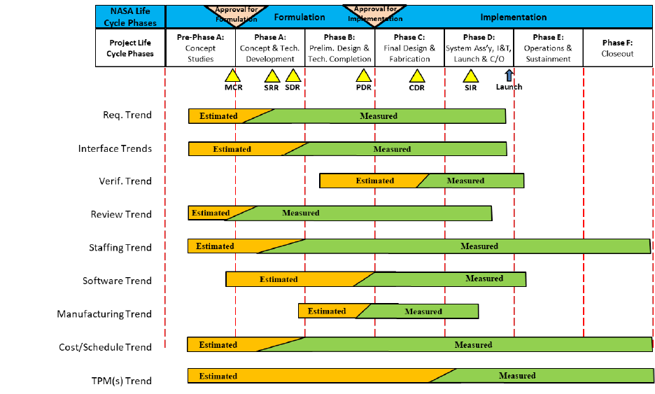
As shown in Figure 2-1, leading indicators are used throughout the program/project life cycle. However,
any one indicator may be useful only during a few of the phases. For example, verification trends are
useful only during the times leading up to and during the phases in which the product is verified. Also, note
that the leading indicators may exist first in an estimated form and then, as more information becomes
available, they may be refined or converted into actual measured values. For example, early in Pre-Phase A
the number of requirements can be estimated and tracked. As the set of requirements is being defined in
Phase A, they can be counted and the actual number can replace the estimated values in the indicators.
6
Figure 2-1 Use of Leading Indicators Throughout the Life Cycle
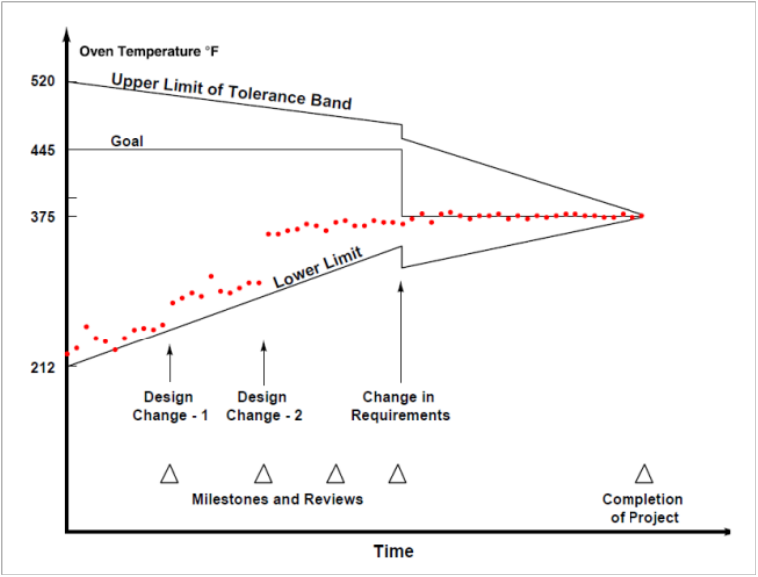
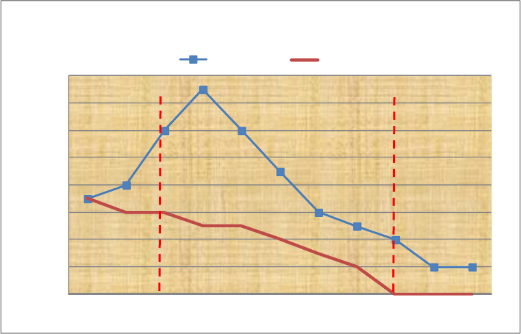
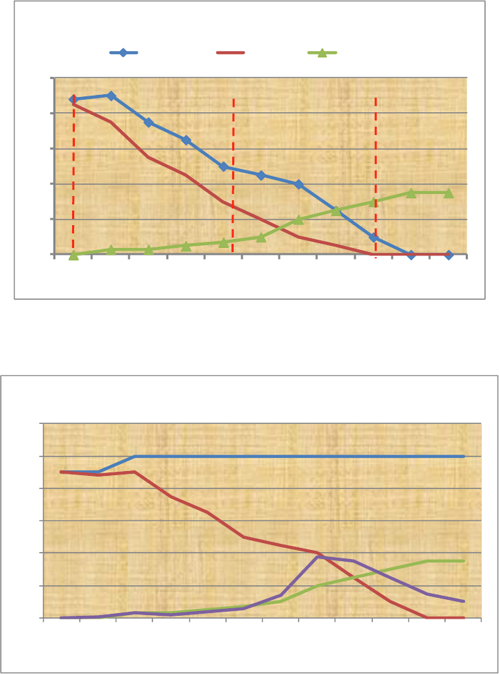
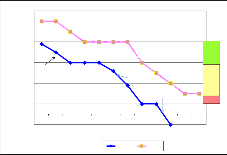
Leading indicators are always viewed against time to see how the measure is progressing so that the
product’s stability and maturity can be determined. This may be depicted in tabular form or perhaps more
usefully in graphical form. The parameters also may be plotted against planned values and/or upper or
lower limits as shown in Figure 2-2. These limits, if used, would likely be defined by the program/project
based on historical information.
By monitoring these trends, the program or project managers, systems engineers, other team members,
and management can more accurately assess the health, stability, and maturity of their program/project.
Trend analysis can help predict future problems that might require attention and mitigation before they
become too costly. How often these parameters should be measured and tracked will depend on the
length, complexity, and size of the program/project. The updated measurements may be provided weekly,
monthly, or quarterly. It is recommended that measurements be taken at least quarterly. However, this
may be too long a period for some projects to catch potential problems in a timely manner. The interval of
measurement for each of the indicators should be identified early in the planning phases and noted in the
Program/Project Plan or other documentation.
7
Figure 2-2 Example Trend Plot from BAE Presentation “Technical Performance Measure,” Jim Oakes, Rick
Botta, and Terry Bahill
By combining these periodic trending indicators with the life-cycle review entrance and success criteria,
the program/project will have better insight into whether their products are reaching the right maturity
levels at the right points in the life cycle, as well as an indication of the stability of the program/project.
The entrance criteria, in particular, address the maturity levels of both the end product as well as the
project documentation that captures its design, development, planning, and risks. However, just looking at
maturity levels is not sufficient. If, for example, the product is appropriately designed to a Critical Design
Review (CDR) maturity level but there are still significant changes in the requirements, the project cannot
be considered stable. An evaluation of the aggregate set of indicators is needed to develop an overall
understanding of both the maturity and stability of the program/project.

8
Common Technical Leading Indicators
A recommended set of common Technical Leading Indicators (TLI) are described in this section. The
common Programmatic Leading Indicators (PLI) are described in Section 4.0. Each section discusses
applicable trend categories, explaining why trends in each category are important and describes the
specific trend measurements that need to be monitored. Each measurement is described, and sample
plots shown. Note that these are only examples. These indicators may be portrayed by the project in the
format that is most useful to the project. The complete set of Common Technical Leading Indicators is
presented in Appendix C along with the minimum characteristics for the displays. As long as the minimum
set of plotting characteristics is satisfied, how the project chooses to depict the trend is left up to the
project and its decision authorities.
3.1. Requirement Trends
This category includes three trends that should be monitored to assess the stability and maturity of the
products: Percent Requirement Growth, To be Determined/To Be Resolved (TBD/TBR) Closures, and the
Number of Pending Requirement Changes. Each is separately discussed in the following sections.
3.1.1. Why Are the Leading Indicators Important?
Controlling the growth of requirements is one of the best ways to reduce unplanned cost and schedule
delays later in a project life cycle. For each new requirement that is added, dozens more may be derived as
the project moves deeper into the product hierarchy. Each of these new and derived requirements will
then need to be verified, again potentially adding more cost and schedule time. Therefore, creating or
defining new requirements must be performed with care. Ensure that each requirement is truly “required”
and not just a desire or wishful thinking. Requirements should convey only those things that absolutely
must happen to produce a product that will accomplish the desired outcome. They should not dictate a
single solution nor strangle the creativity of the designer. The requirement set should allow for multiple
design options that can then be traded against key parameters such as performance, cost, and schedule.
Depending upon where the project is in the life cycle, requirement growth is not necessarily a bad thing.
During Phase A, the project moves from having no requirements to the formal definition of the
requirements culminating with the System Requirement Review (SRR). So naturally, there should be a
drastic increase in requirements. Also within phase A is the System Definition Review (SDR) at which the
architectures are presented. It is also expected that there may be additional requirements defined during
this part of the life-cycle phase.
As the project moves to Phase B and the Preliminary Design Review (PDR), the requirement growth or
velocity should be significantly slowed but realistically may see some small growth as the designs are
prototyped, gaps in the requirement set are found, unforeseen need for a requirement is identified, etc. As
the project moves into Phase C and the Critical Design Review (CDR) and the product design is finalized,
requirement growth should be very small. The later requirements are added to a project, the more difficult
they may be to enact and the more cost and schedule they may be adding. As the project completes Phase
9
C, culminating with the System Integration Review (SIR) and moves into Phase D, requirements growth
should be virtually zero. Adding significant requirements at this point will likely mean scrapping previously
designed parts and starting a redesign cycle.
3.1.2. Percent Requirement Growth Trend Description
This indicator provides insight into the growth trend of the program/project’s requirements and their
stability. Requirements growth, sometimes called “requirements creep,” can affect design, production,
operational utility, or supportability later in the life cycle. For each requirement added, there is a
corresponding cost of time and schedule involved for its handling, maintenance, and verification. The basic
question being answered by this indicator is “Is the program/project effort driving towards requirements
stability?”
Base measurement for this indicator is the total number of requirements in each of the program/project’s
requirement documents. The program/project first determines where all its requirements are located and
how far down within the product hierarchy the requirements will be tracked. For example, there may be
several layers of requirements as they flow down to systems, subsystems, elements, assemblies, and
components within the overall project. Some requirements will be the responsibility of the NASA
program/project team; some requirements may be the responsibility of a contractor or vendor. The
program/project will need to decide how far down it is practical to determine this metric. How far down
they will be tracking requirements should be part of the discussion in their Formulation Agreement and/or
Program/Project Plan on how they will provide this indicator.
Since most program/projects use a tool to help keep track of their requirements (Cradle, DOORS, Excel
spreadsheet, Word document, etc.), counting should be a simple matter of asking the application they are
being stored in how many there are or how many times the word “shall” appears in their document. This
can be automated in many cases. This assumes that the program/project is following good requirements
definition practices of only using “shalls” to define a requirement and that there is only one “shall” per
requirement. The practice of having one sentence with a “shall” to introduce a number of requirements
(e.g. “The product shall perform the following characteristics: a. Breathable atmosphere for 30 days b.
continuous pressure of 8.1 psia, etc.) is not used or if it is used that each of these obscured requirements is
numbered. A spreadsheet that keeps track of these measurements might be as shown in the first and
second column of Table 3-1 (the third column will be discussed in the next section). This would be a
representation for a snapshot of the number of requirements on a certain date. Other snapshots would be
taken periodically and results tracked over time.
10
Table 3-1 Simple Snapshot Requirement Tracking Spreadsheet
The first column lists the documents within the project that contain requirements. The project has decided
to track requirements at the project, system, subsystem, and ICD level (more about ICDs will be discussed
in later sections). The second column captures what date the count was taken, and the third column
captures how many requirements were in the document at that date. This information would be taken
periodically at an interval that makes sense for the program/project. It must also be decided whether to
track the requirements at the individual document level and/or in total of all the documents. Again, this
strategy should be included in the Formulation Agreement or Program/Project Plan.
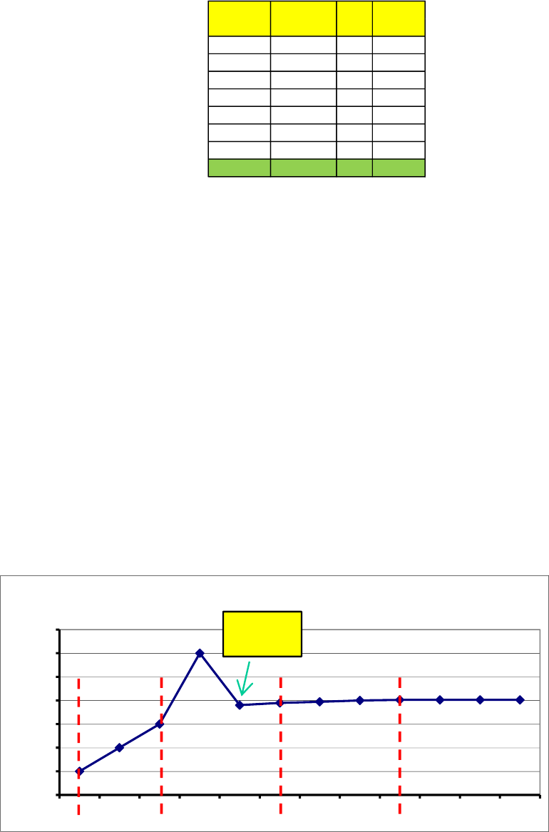
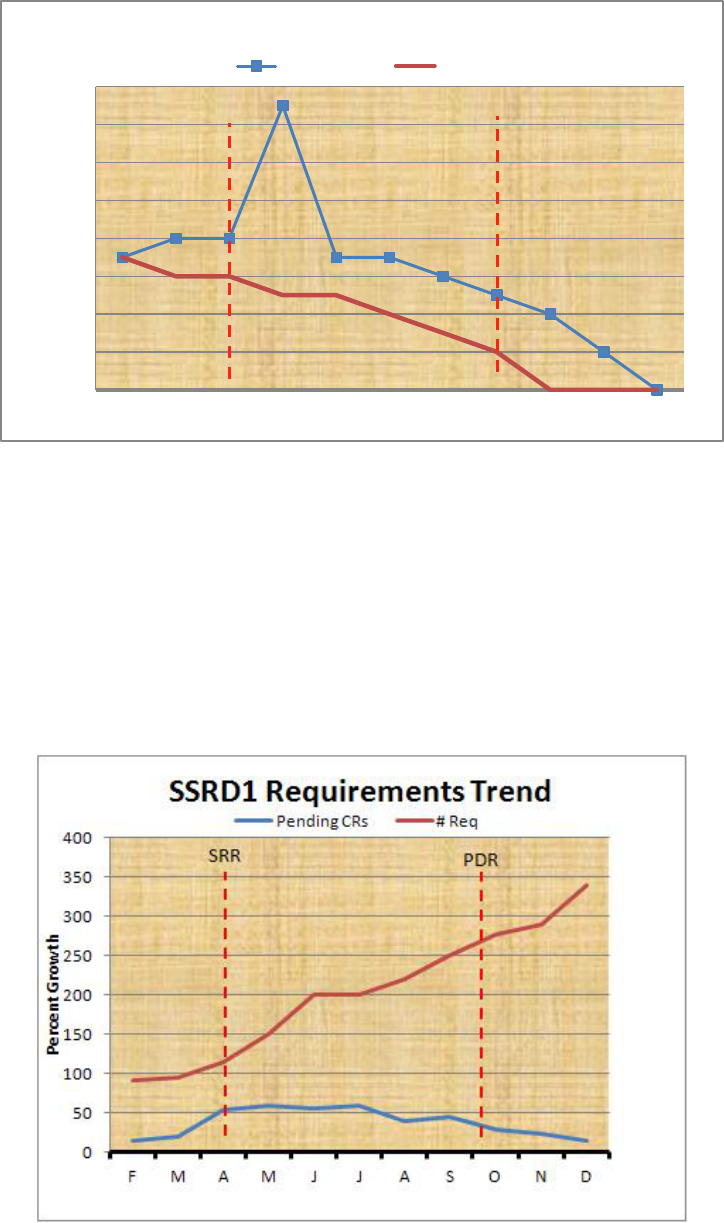
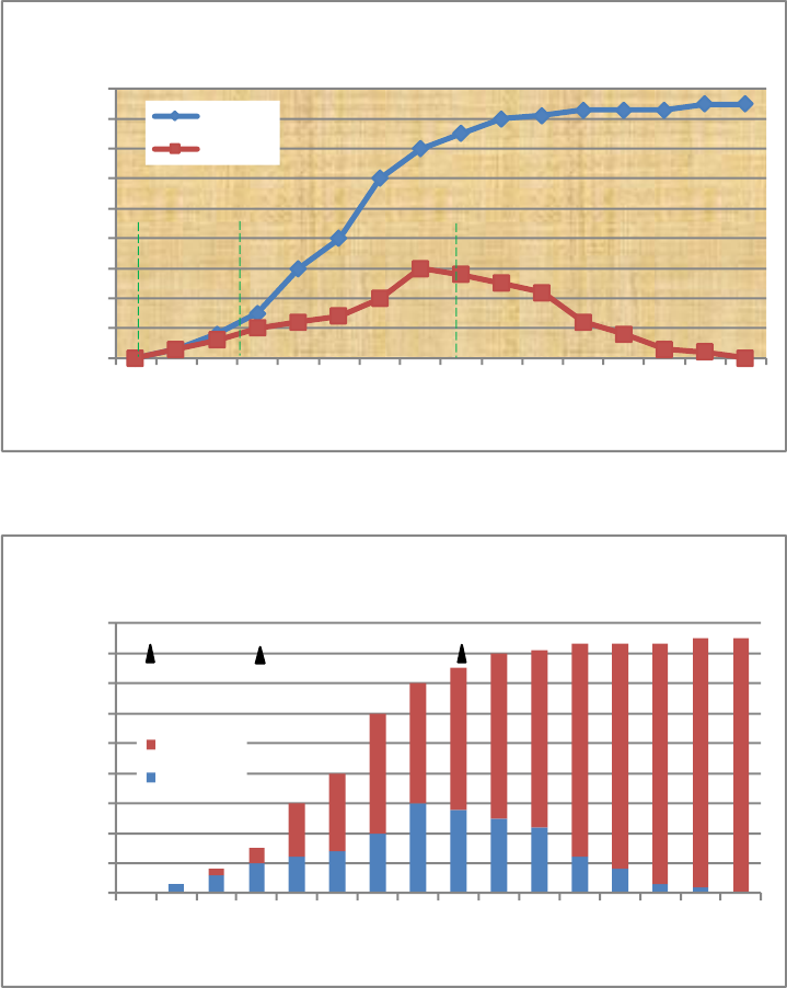
As these requirement snapshots are built up over time, they can then be tabularized and plotted. Figure 3-
1 is a simple plot of requirements using raw number of requirements—this could be per document or as a
total for the project. For this type of graph, it is not the raw number of requirements that is of interest
(large projects may have many requirements while small project may have few), it is the shape of the
curve that indicates how the number is growing or has become stable. It is useful to include notes about
unusual characteristics on the graph—in this case a requirement scrub activity was noted to bring the
number of requirements back into control. It is also good to put key milestones such as life-cycle reviews,
on the graph so that the data can be evaluated within context.
Figure 3-1 Simple Requirements Growth Plot – Raw Count
PRD xx/xx/xx 90
5
SRD xx/xx/xx 150
8
SSRD 1 xx/xx/xx 300
15
SSRD 2 xx/xx/xx 200
10
ICD 1 xx/xx/xx 25
5
ICD 2 xx/xx/xx 53
20
ICD 3 xx/xx/xx 16
3
Total 834
66
Document
Date
# Req
# TBD/
TBRs
Requirements Growth Trends
0
50
100
150
200
250
300
350
Jan Feb Mar Apr May Jun Jul Aug Sep Oct Nov Dec
Number of Requirements
SRR
PDR
CDR
SAR
SRD
Requirement
scrub
11
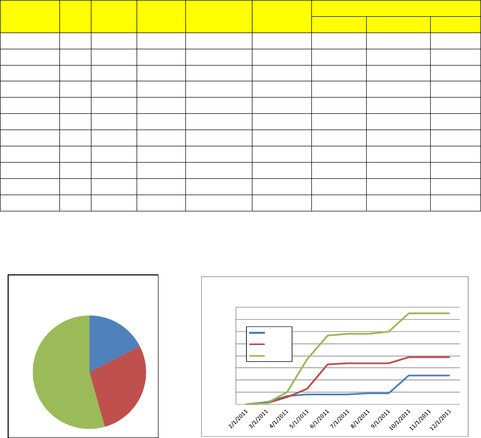
Another way of plotting this information is in the percentage of growth since the last measurement period.
Table 3-2 shows an example spreadsheet for the requirements within a single document, say SSRD1 from
the above spreadsheet.
Table 3-2 Simple Spreadsheet for Percent Requirements Growth
Date
#
Req
% Req
Growth
2/1/2011
92
0%
3/1/2011
96
4%
4/1/2011
115
20%
5/1/2011
150
30%
6/1/2011
110
–27%
7/1/2011
112
2%
8/1/2011
113
1%
9/1/2011
115
2%
10/1/2011
80
–30%
11/1/2011
80
0%
12/1/2011
80
0%
The percent growth is calculated by subtracting the number of requirements on a date from those on its
previous date and dividing by the number of requirements on the previous date and then multiplying by
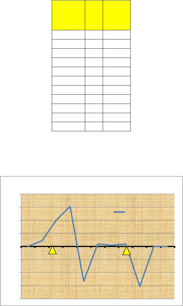
100 (e.g., (96-92)/92 x 100 = 4%). When plotted the data would look like Figure 3-2:
Figure 3-2 Simple Requirements Growth Plot
-40%
-30%
-20%
-10%
0%
10%
20%
30%
40%
F
M
A
M
J
J
A
S
O
N
D
Requirements Growth
% Req Growth
SRR
PDR
12
As can be seen, the requirements were growing up through SRR as expected, but then continued to grow
thereafter. At some point a requirements scrub took place and so the requirements growth went negative
and then stabilized until just after PDR when some requirements were deleted and then remained stable
again.
So the question is—is this a “good” project or not? In the ideal model, requirements would grow through
SRR at which time all requirements would be perfectly defined and then growth would be zero thereafter.
In the real world, this rarely happens. As concepts are refined, designs deepened, and the realities of the
political and budgetary changes affect the projects, it is customary to see requirements grow and ebb.
After SRR, it is always desirable to keep requirements growth to a minimum, but some change is to be
expected. It is clear that in the project example shown in Figure 3-1, requirements have continued to grow
well after PDR. This should trigger a flag that a closer look at the requirements situation is warranted. This
might be completely explainable but at least the trend would indicate that more attention might need to
be paid to the situation. As historical data is gathered across multiple projects, guidelines or upper/lower
boundary conditions can be developed against which this data could be plotted. Some Centers or projects
may already have this type of boundary information available and if so, plotting against predictions or
plans would be very useful.
3.1.3. TBD/TBR Closures Trend Description
As noted in Table 3-1, another useful indicator is the number of “to be determined” (TBD) or “to be
resolved” (TBR) requirements within each document. TBDs/TBRs are used whenever the project knows
they need a requirement for some performance level but may not yet know exactly what that level is.
Typically, a TBD is used when the level has not been determined at all, whereas a TBR is used when a likely
level has been determined but further analysis or agreements need to be obtained before setting it
officially as the requirement level. Additional analysis, prototyping, or a more refined design may be
required before this final number can be set. As the project moves later in the life cycle, remaining
TBDs/TBRs hold the potential for significant impact to designs, verifications, manufacturing, and
operations and therefore present potentially significant impacts to performance, cost, and/or schedule.
Typically, this indicator is viewed as a “burndown” plot, usually against the planned rate of closures. An
Example is shown in Figure 3-3.
13
Figure 3-3 TBD/TBR Burndown
3.1.4. Number of Pending Requirement Changes Trend Description
In addition to the number of requirements that are already in the program/project documentation, there
are usually a number of potential changes that may be working their way through the requirements
management process. Keeping up with this bow wave of potential impacts is another way of analyzing the
requirements indicator trend. The number of pending change requests can be plotted along with the
previous requirement trend graphs as shown in Figure 3-4.
Figure 3-4 Pending Requirement Change Requests
0
2
4
6
8
10
12
14
16
F M A M J J A S O N D
Number TBD/TBRs
TBD/TBR Burndown
# TBD/ TBRs Plan
SRR
PDR
14
The program/project may elect to keep track of additional information. One useful indicator is the reason
for the change—is it a new requirement that is being driven by sources external to the project and
therefore not within their control? Is it driven by the customer adding new requirements and therefore
the customer should expect a potential increase in cost and/or schedule? On the other hand, is it a
requirement that the project just missed or did not realize they needed and therefore represents an
internal change that may need to be justified to the customer (especially if it involves a cost/schedule
increase)? Table 3-3 shows a more complete spreadsheet that keeps up with this rationale as well as the
previous spreadsheets for number of requirements, number of TBD/TBRs, and the percent growth
indications.
Table 3-3 Requirement Changes and Reason
Date
#
Req
# TBD/
TBRs
% Req
Growth
% TBD/TBR
Growth
No. Req
Changes
Reason
External
Customer
Internal
2/1/2011
92
7
0%
0%
0
0
0
0
3/1/2011
96
8
4%
14%
4
2
1
1
4/1/2011
115
8
20%
0%
19
5
5
9
5/1/2011
150
15
30%
88%
35
1
7
27
6/1/2011
110
7
– 27%
–53%
–40
0
20
20
7/1/2011
112
7
2%
0%
2
0
1
1
8/1/2011
113
6
1%
–14%
1
1
0
0
9/1/2011
115
5
2%
–17%
2
0
0
2
10/1/2011
80
4
–30%
–20%
–35
15
5
15
11/1/2011
80
2
0%
–50%
0
0
0
0
12/1/2011
80
0
0%
–100%
0
0
0
0
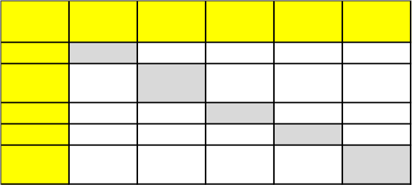
A snapshot plot of this information could be generated as shown in Figure 3-5 or a trend line graph
developed as shown in Figure 3-6. There are many ways to represent this information.
Figure 3-5 Change Source Snapshot Figure 3-6 Change Source Trend
External
18%
Customer
28%
Internal
54%
Req Growth Driver
0
10
20
30
40
50
60
70
80
No. Req Changes (Cum)
Requirement Change Source
Internal
Customer
External

15
Some projects may want to maintain additional information about each requirement change, such as the
cost and schedule impacts. Table 3-4 is an example of additional information that may be useful.
Table 3-4 Additional Data for Understanding Requirement Changes
Require-
ment
Req. Change
Impact
Reason
Status
Added
(New)
Deleted
Modified
Cost
Sched
External
Customer
Internal
SRD # 42
X
$3M
6 mo.
X
Approved
ICD 1004
Req. 14.1
X
– $90K
– 8 mo.
X
Pending
PRD
Req. 45
X
0
0
X
Approved
3.2. Interface Trends
This category of trends includes the percentage of ICDs that have been approved, the burndown of
TBDs/TBRs within those documents, and the number of interface change requests.
3.2.1. Why is the Leading Indicator Important?
This indicator is used to evaluate the trends related to growth, stability, and maturity of the definition of
system interfaces. It helps in evaluating the stability of the interfaces to understand the risks to other
activities later in the life cycle. Inadequate definition of the key interfaces in the early phases of the life
cycle can drastically affect the ability to integrate the product components in later phases and cause the
product to fail to fulfill its intended purpose. The longer these interfaces are left undefined, the more likely
problems will occur and therefore negative impacts to performance, cost, and schedule.
Interface requirements may be contained in various documents depending upon the program/project.
Some program/projects will define them at a high level in an Interface Requirements Document (IRD).
These may be taken by the subsequent engineering teams, (often a prime contractor, or vendor) to be
further detailed as an ICD. If a program/project is interfacing to a legacy system, they may be working to
what is often called a “one-sided ICD” or an Interface Definition Document (IDD). Other programs/projects
may put the high level and/or detailed interface requirements and agreements into other documents. For
simplicity, the term ICD will be used here, but it is intended to be whatever document(s) contain the
interface requirements and definitions for the program/project.
Note that the requirements within the interface documents as well as the number of requirement TBDs
and TBRs need to be included with the overall requirement trend as discussed in section 3.1.1. However,
the program/project may also choose to account for the interface-related requirements trends separately
16
from the non-interface related requirements due to their importance. How the accounting is made needs
to be clear in the Formulation Agreement and/or Program/Project Plan.
3.2.2. Percent ICDs Approved
The program/project will need to identify how many documented interfaces it needs both between
elements within their system as well as to the interfacing elements external to their product. Once the
total number of interface documents has been identified, this indicator will reflect trends in their approval.
One way of capturing where interfaces exist within a system, what kind of interfaces they are (bottom left
half) and where the interface definition and requirements are documented (upper right half) is shown in
Table 3-5.
Table 3-5 Example Matrix for the Identification of Interfaces for a Program/Project
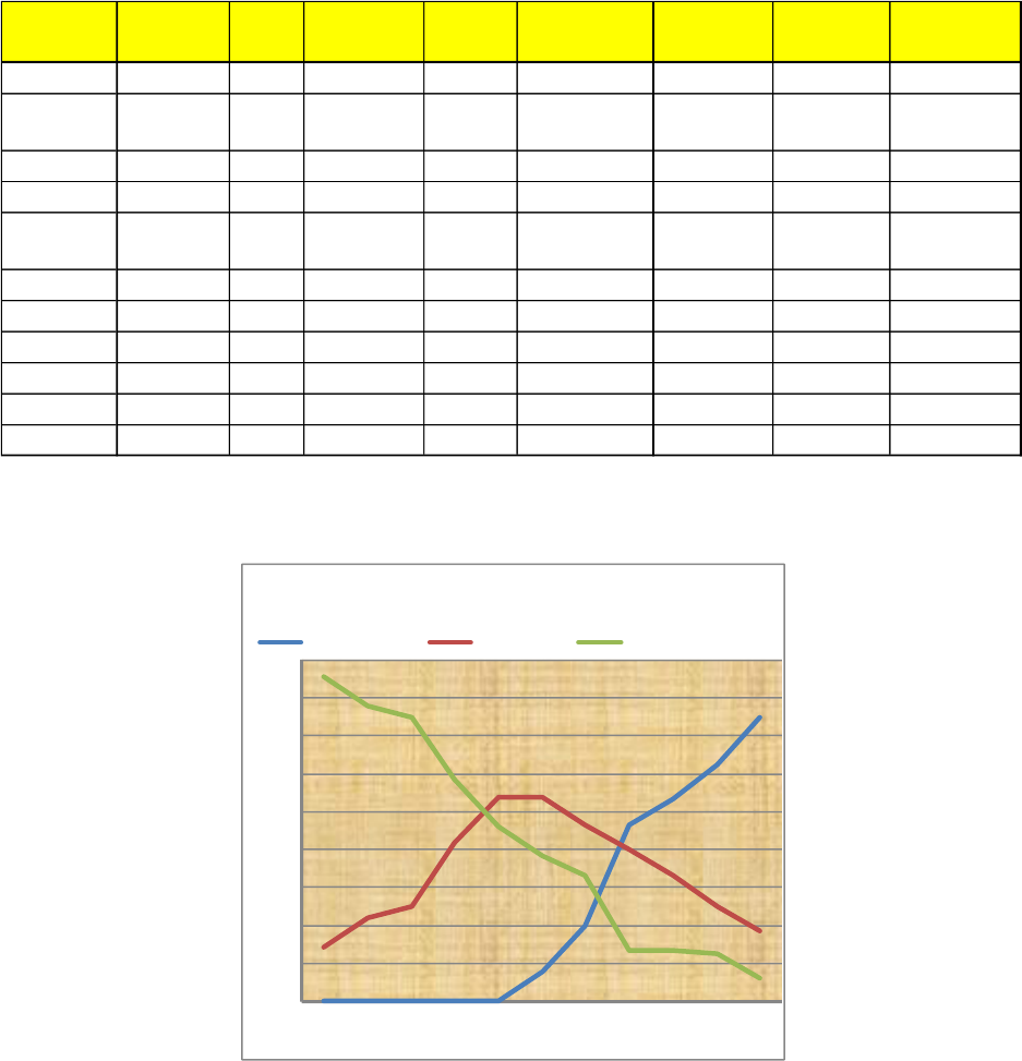
Once the interfaces are determined, a program/project can track how many of them have been developed
and approved. For programs/projects with few interfaces, this can be done in a tabular form as shown in
Table 3-6 for example. Programs/projects with many interfaces may want to display the trend graphically
as shown in Figure 3-7.
ICDs Element 1 Element 2 Element 3 Element 4 Element 5
Element 1 ICD 1 ICD 2 ICD 3
Element 2
Data,
Fluid
Drawing 1
Element 3 Power None IDD 1
Element 4 None Data None
Element 5
Data,
Power
None
Fluid,
Power
None
17
Table 3-6 Example of Tabular Tracking of Interface Documents
Figure 3-7 Example Plot Trending Interface Documentation
3.2.3. ICD TBD/TBR Burndown
In addition to the requirements TBD/TBRs that are discussed in Section 3.1.3, there may be others within
the interface documentation. This indicator will track them. The program/project may elect to lump them
together with the requirement TBD/TBRs if desired. Similar tracking is done as for the requirement
# ICDs Planned Actual # Approved
# In
work
# Not Started
%
Approved
% In work
% Not
Started
2/1/2019
7 7 0 1 6 0% 14% 86%
3/1/2019
7 9 0 2 7 0% 22% 78%
4/1/2019
7 12 0 3 9 0% 25% 75%
5/1/2019
8 12 0 5 7 0% 42% 58%
6/1/2019
8 13 0 7 6 0% 54% 46%
7/1/2019
9 13 1 7 5 8% 54% 38%
8/1/2019
9 15 3 7 5 20% 47% 33%
9/1/2019
9 15 7 6 2 47% 40% 13%
10/1/2019
9 15 8 5 2 53% 33% 13%
11/1/2019
10 16 10 4 2 63% 25% 13%
12/1/2019
10 16 12 3 1 75% 19% 6%
0%
10%
20%
30%
40%
50%
60%
70%
80%
90%
F
M
A
M
J
J
A
S
O
N
D
Number of ICDs
% Approved
% In work
% Not Started
18
TBD/TBRs in Section 3.1.3 and plotting the information can be made in several ways. A simple example is
shown in Figure 3-8.
Figure 3-8 Example ICD Non-Requirement TBD/TBR Burndown vs. Plan
3.2.4. Number of Interface Change Requests
Similar to the need to track requests for changes to the program/project requirements, tracking change
requests to the interface documentation is also an indication of a pending set of changes that might affect
the future performance, cost, and schedule. As these changes come later in the life cycle, they may affect
agreements or designs that have already started in the manufacturing process. Changes coming this late in
the life cycle can affect many organizations, requiring redesign, scrapping of parts, and recertification.
Like the requirements change requests discussed in Section 3.1.4, similar information may be gathered
about the interface change requests. For example, Table 3-7 shows an example of the information that
might be gathered. In addition, the cost or schedule impact and status of the requests also may be
gathered and plotted.
0
2
4
6
8
10
12
14
16
F
M
A
M
J
J
A
S
O
N
D
Number TBD/TBRs
ICD Non-Requiremnt TBD/TBR Burndown
# TBD/ TBRs
Plan
SRR
PDR
19
Table 3-7 Example Information for Interface Trending
3.3. Verification Trends
Verification of a program/project’s product is the proof of compliance with its requirements. This is done
through test, analysis, demonstration, or inspection. Each requirement will need to be verified through
one or more of these methods. This category includes two indicators: verification closure burndown and
the number of deviations/waivers requested as a result of the verification activities.
3.3.1. Why is the Leading Indicator important?
Tracking which requirements have and have not been verified can be accomplished through various means
as appropriate for the size and complexity of the program/project. Complex programs/projects may use a
tool such as CRADLE or DOORs, others may use spreadsheets or word documents. Whatever method is
chosen, it is important to know which requirements have been verified (i.e., “closed”) and which are still to
be verified (“open”). This can be indicated by flags or other indicators within a selected tracking tool, using
separate Verification Closure Notices (VCN), or other means chosen by the program/project.
Leaving verification closure too late in the life cycle increases the risk of not finding significant design issues
until the cost of correcting them is untenable. Often, this means additional cost and schedule to correct
the problems or having to work around the problems through more complex operational scenarios.
External Customer Internal
2/1/2011 15 7 0% 0% 0 0 0 0 7
3/1/2011 15 8 0% 14% 0 2 1 1 6
4/1/2011 20 12 33% 50% 5 5 5 9 6
5/1/2011 30 15 50% 25% 10 1 7 27 5
6/1/2011 50 12 67% -20% 20 0 20 20 5
7/1/2011 60 9 20% -25% 10 0 1 1 4
8/1/2011 62 6 3% -33% 2 1 0 0 3
9/1/2011 65 5 5% -17% 3 0 0 2 2
10/1/2011 80 4 23% -20% 15 15 5 15 0
11/1/2011 80 2 0% -50% 0 0 0 0 0
12/1/2011 80 2 0% 0% 0 0 0 0 0
Delta I/F
Date
# I/F
# TBD/
TBRs
%
Interfac
% TBD/TBR
Growth
Reason
Plan
20
3.3.2. Verification Closure Burndown
This indicator tracks the closure of the requirement verifications as an indication of project maturity and
stability. Table 3-8 is an example of the parameters a program/project may track over time. This
information can be displayed graphically as either numbers or percentages of open verifications. It is useful
to plot them against a predicted or planned rate of closure for better insight as shown in Figure 3-8.
Table 3-8 Example Matrix for Tracking Verification Closure Burndown
Figure 3-8 Example Plot of Verification Burndown
1/1/19 90
90 0 100% 90 100% 0
2/1/19 90
88 2 98% 85 94% 0
3/1/19 100
90 10 90% 75 75% 3
4/1/19 100
75 25 75% 55 55% 3
5/1/19 100
65 35 65% 45 45% 5
6/1/19 100
50 50 50% 30 30% 7
7/1/19 100
45 55 45% 20 20% 10
8/1/19 100
40 60 40% 10 10% 20
9/1/19 100 25 75 25% 5 5% 25
10/1/19 100 10 90 10% 0 0% 30
11/1/19 100 0 100 0% 0 0% 35
12/1/19 100 0 100 0% 0 0% 35
#
Waivers
# Planned
Open verif.
% Planned
Open verif.
Date
# Verif
open
verif.
Closed
verif.
% Open
verif.
0%
20%
40%
60%
80%
100%
120%
J
F
M
A
M
J
J
A
S
O
N
D
Percent of Open Verifications
% Open verif.
"Planned"
CDR
SIR
SAR
21
3.3.3. Number of Deviations/Waivers Approved/Open
A waiver or deviation is a documented agreement intentionally releasing a program/project from meeting
a requirement. The standard definition of a deviation is alleviating a program/project from a requirement
before the set of requirements are baselined and a waiver is after the requirements are baselined. Some
programs/projects make the distinction that a deviation is granted when the program/project is in the
Formulation Phases (Pre-Phase A, Phase A, Phase A or Phase B) and a waiver when in the Implementation
Phases (Phase C, D, E, or F). In either case, it is important to document and track both the approved and
pending requests. Increasing numbers of deviations/waivers may indicate potential issues later in the life
cycle as the product begins to vary from the set of requirements deemed necessary to satisfy the customer
and other stakeholders.
Table 3-9 is an example spreadsheet of how these indicators might be tracked. The program/project may
choose to gather and track other information about the waivers such as the reason, who submitted, cost if
not approved, etc.
Table 3-9 Example Tracking of Approved and Pending Waivers
This information also can be plotted against the verification closures to give a more complete picture of
the verification activities as shown in Figure 3-9. Figure 3-10 shows an example of another important
parameter to track—the number of waivers/deviations that have been requested but not yet
dispositioned (i.e., “pending”). This may represent a bow wave of waivers that could affect future cost and
schedules.
Date 1 90
90 0 0
Date 2 90
88 0 1
Date 3 100
90 3 3
Date 4 100
75 3 2
Date 5 100
65 5 4
Date 6 100
50 7 6
Date 7 100
45 10 14
Date 8 100
40 20 38
Date 9 100 25 25 35
Date 10 100 10 30 25
Date 11 100 0 35 15
Date 12 100 0 35 10
Date
# Verif
Open
Verif
#
Approved
Waivers
#
Waivers
Pending
22
Figure 3-9 Example Plot of Waivers Granted and Verification Burndown
Figure 3-10 Example of Waivers Approved and Pending
3.4. Review Trends
This indicator tracks the activities resulting from a life-cycle review. Depending on the program/project,
the items that are identified for further action by the reviewing body may be called Action Items (AI),
Requests for Action (RFA), Review Item Discrepancies (RID) or other nomenclature. Whatever they are
called, it is important to track their disposition and eventual closure. There is one indicator in this category:
RID/RFA/AI burndown per review
0
20
40
60
80
100
J
F
M
A
M
J
J
A
S
O
N
Number of Open Verifications
open verif.
Planned
"Waivers"
CDR
SIR
SAR
0
20
40
60
80
100
120
J
F
M
A
M
J
J
A
S
O
N
D
Number of Waivers
# Total Verifications
Open Verif.
Approved Waivers.
Pending Waivers.

23
3.4.1. Why is the Leading Indicator Important?
The purpose of a life-cycle review is to reveal the work of the program/project during that phase of the life
cycle to a wider audience so that any issues, problems, design deficiencies, clarification of interpretations
are presented and general buy-in by the stakeholders may be obtained. These comments (RFAs, RIDs, AI,
etc.) are usually gathered and then dispositioned in some way. Some comments may not be valid or may
be out of scope and so may be rejected. Some comments may be approved as is or modified in some way
that is acceptable to both the submitter and the program/project. Those that are approved will need to be
executed and the agreed-to work accomplished. At that point, the submittal is considered “closed.”
While closing some comments may need to wait for a key triggering activity, not closing review comments
in a timely manner may be pushing work off later and later in the life cycle where its implementation could
have a cost and schedule impact. Critical design issues may be dragging on, which could affect subsequent
design, manufacturing, testing, and/or operational activities. While some of these issues may be very
tough and contentious, it is always better to face them as early as possible and drive to an agreed-to
solution.
Note that another related indicator, life-cycle review date slippage, is addressed in the Schedule Trend
section with the life cycle being one of several key milestones. (See Section 4.2.)
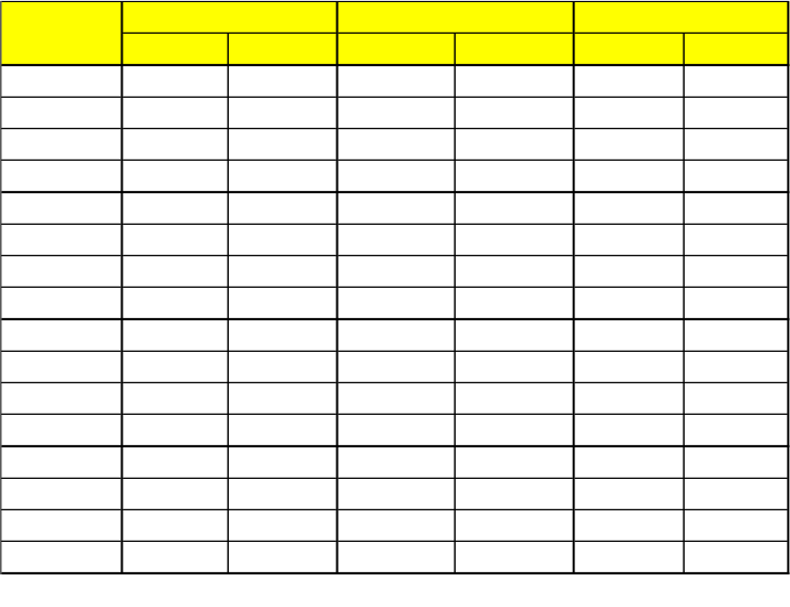
3.4.2. RID/RFA/Action Item Burndown per Review
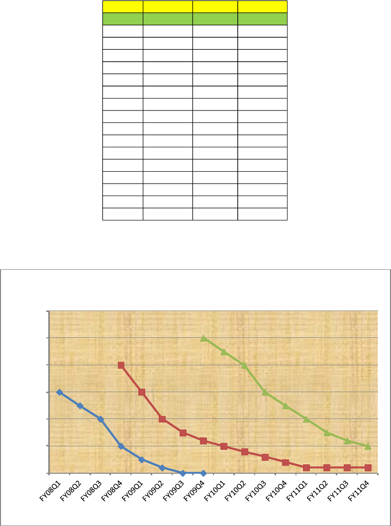
This indicator is required per NPR 7123.1. Table 3-10 shows an example spreadsheet that is tracking the
number of RID/RFA/AIs for a given life-cycle review. Note this measure is gathered periodically, in this case
quarterly, not just at the next life-cycle review. Trending works best if the measurements are taken
regularly.
24
Table 3-10 Number of Open RFAs/RIDs/AIs per Review
This information perhaps can be better seen graphically. Figure 3-11 is an example.
Figure 3-11 Number of Open RFAs/RIDs/AIs per Review
Date MCR SRR PDR
Total 35 40 55
FY16Q1 30
FY16Q2 25
FY16Q3 20
FY16Q4 10 40
FY17Q1 5 30
FY17Q2 2 20
FY17Q3 0 15
FY17Q4 0 12 50
FY18Q1 10 45
FY18Q2 8 40
FY18Q3 6 30
FY18Q4 4 25
FY19Q1 2 20
FY19Q2 2 15
FY19Q3 2 12
FY19Q4 2 10
0
10
20
30
40
50
60
Number Open
Open RFA/RIDs/AI
MCR
SRR
PDR
25
3.5. Software-Unique Trends
Software metrics or indicators are used to measure some property of a piece of software—its
specifications, plans, or documentation. While Software Engineering has a rich history and large potential
selection of measures, the single software metric “Number of Requirements/Features per Build/Release
versus vs. Plan” continues the emphasis on requirements compliance measurement early in the
program/project life cycle when it can be of maximum benefit and cost-effectiveness.
3.5.1. Why is the Leading Indicator Important?
This measure is used to evaluate the trends in meeting the required characteristics or features of a specific
software build or release and the overall build/release development plan. Failure to meet the planned
features of a build or release may indicate the inability to support the required development, analysis,
verification, and testing of dependent hardware, software, or systems or of larger, more complex tasks
ahead. A common occurrence on software projects in trouble is inability to meet the requirements and
features of planned builds/releases and deferral of requirements and verifications to later builds/releases.
This metric reveals program/project risk in terms of rework, infeasible schedule, and deferred work to later
builds/releases. It can also mean several other things: the Program/Project may not have planned well
and does not have the productivity they expected; they may be having staffing problems and can't make
their schedules; some of the requirements may still be TBD or unclear or they may be having difficulty
implementing some of them; they could be waiting on hardware deliveries, etc.
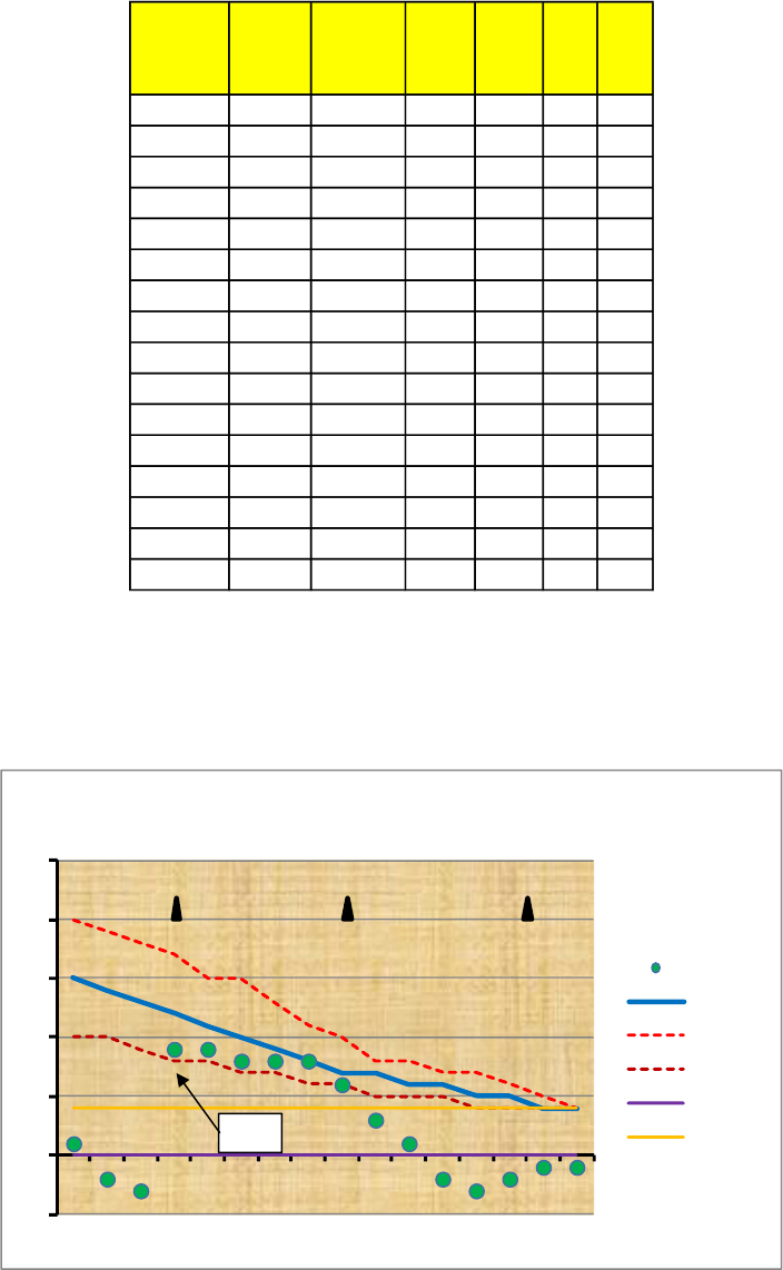
3.5.2. Number of Requirements/Features per Build/Release vs. Plan
This metric/indicator provides a quantitative measure of the number of requirements or features in a build
vs. the number of requirements or features that were planned.
It is illustrated by counting the total number of requirements or features that were planned for each
build/release, counting the total number of requirements or features that were actually included in the
build/release, and then comparing the two to show how well the plan is being met by the development
effort. They can also be linked to major system or software milestones to suggest the overall impact to the
program/project/system.
A simple illustration of this is shown in Table 3-11.
26
Table 3-11, Table of Plan vs. Actual Requirements/Features by Build/Release
Another approach is a more graphic software build trend histogram illustrated in Figure 3-12.
Figure 3-12 Software Build Trend Histogram
Another method of displaying this indicator is shown in Figure 3-13, which links the parameter to
program/project milestones and build version numbers.
Build No.
# Planned
Features
# Features
in Build
0.5 15 10
1.0 50 45
1.1 120 100
1.2 300 230
1.3 300 300
1.4 400 389
1.5 440 415
2.0 600 500
2.1 650 560
3.0 700 610
5
5
20
70
0
11
25
100
90
90
0
100
200
300
400
500
600
700
800
0.5
1.0
1.1
1.2
1.3
1.4
1.5
2.0
2.1
3.0
No. Features
Build Version
SW Build Requirements
# Not Met
# Features in Build
27
Figure 3-13 Percent Features Met per Build Version
3.6. Problem Report/Discrepancy Report Trends
Programs and projects conduct verification, validation, and quality control activities during the
implementation life-cycle phases to ensure requirements and stakeholder expectations will be satisfied in
advance of launch or being sent into the field. Where possible and determined practical, these activities
are conducted in an environment as close to operational as possible, that exercise all the operational
modes and scenarios as fully as possible, and that use the actual flight procedures and databases that will
used during launch and operations. If during the conduct of these activities, the product fails to meet
requirements or accepted standards, the problem is captured, reported to program/project management,
and a corrective action or work around is developed. Depending on the Center, program, or project these
problem identifications may be called problem reports or discrepancy reports.
3.6.1. Why is the Leading Indicator Important?
The systems that are built by NASA are often complex; distributed across people, organizations, and
geography; implemented in multiple releases, builds, and patches; and affected by changes to baseline
requirements approved by a configuration change board during the implementation phases. This
demanding environment means that virtually no system is ever delivered without discrepancies, i.e.,
deviations from expected and/or required performance. The programs/projects are required to capture
these discrepancies and compile the information so corrective action can be documented. When
normalized against the project complexity, discrepancy reports can be used as a predictor of system
performance. This leading indicator is applicable to both hardware and software projects.
0%
20%
40%
60%
80%
100%
120%
0.5
1.0
1.1
1.2
1.3
1.4
1.5
2.0
2.1
3.0
Build Version
Percent Features Met per Build
PDR CDR SIR

28
In order to offer the most accurate predictor of future performance of the system being verified it is
important that the discrepancy process be applied across all parties involved. This means both government
and commercial suppliers should be required to participate in the process often requiring a single
synchronized reporting timeline be used. Additionally, supporting information intended to characterize a
discrepancy and document its history should be included in the regular reporting process.
3.6.2. Number of Discrepancy Reports (DRs) Open, Total Number of DRs
Depending on the specific project, there will be multiple types of discrepancy report information available
for evaluation. Projects are encouraged to use this information to improve visibility into the actual
condition of the system being developed. As a minimum, all projects should utilize a minimum of two data
types in their regular reporting process: 1) number DRs/Problem Reports (PRs) open and 2) total number
DRs/PRs.
This information is used to evaluate trends in the rate of closure and closure percentage of PRs and/or
DRs. Large deviations for the planned closures of DRs/PRs vs. the schedule defined at the start to address
them may be indicative of:
• Work not being completed as planned – in certain cases, the project team may be focused on
commitments to deliver new functionality and not have the resources to address DR
remediation in the workflow.
• Low quality of re-work – workmanship issues, problem parts, flawed fabrication steps are
examples of problem sources that will result in frequent re-work despite the best efforts of a
project to repair the problems the first time.
• Insufficient resources – Negative trends associated with DRs may be symptomatic of project
resources becoming strained. This may be due to incorrect assumptions regarding the
complexity of the solutions needed to resolve the problems; optimistic planning of workforce
levels or workforce skill mix used to address the discrepancies found plus new ones entering
the system; or insufficient resources (i.e., time and/or schedule) allotted for regression testing
of fixes before the DR can be closed.
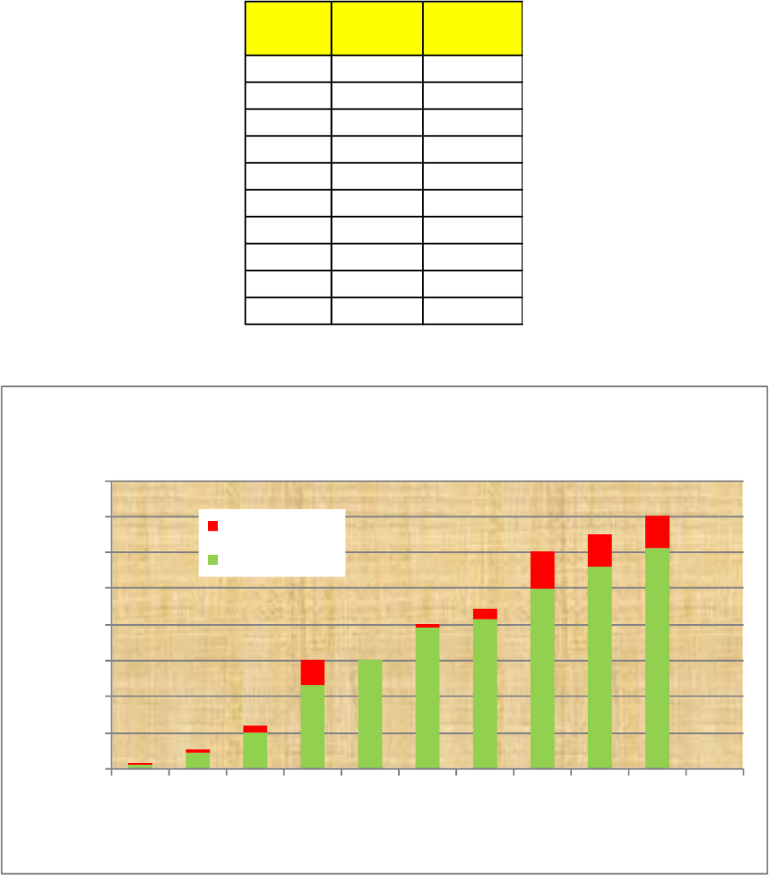
Figures 3-14 and 3-15 illustrate report formats that could be used to track project DRs and PRs. In
preparing the specific format to be employed on the project, consider showing progress on closing PR/DRs
vs. time, indicating key life-cycle milestones for reference, and including descriptions of these key
milestones to ensure an accurate understanding across all stakeholders.
29
Figure 3- 14 DR/PR Closures Over Time
Figure 3-15 DR/PR Trend as Stacked Percentage
3.7. Technical Performance Measures
According to NPR 7123.1, TPMs are the set of critical or key performance parameters that are monitored
by comparing the current actual achievement of the parameters to that anticipated at the current time
and on future dates. They are used to confirm progress and identify deficiencies that might jeopardize
meeting system requirements. Assessed parameter values that fall outside an expected range around the
anticipated values indicate a need for evaluation and corrective action. There are two types of TPMs
discussed in this section: the required common TPMs of mass margin and power margin and the other
project unique TPMs (the selection of which will depend upon the type of product the program/project is
producing).
0
10
20
30
40
50
60
70
80
90
1/1/18
2/1/18
3/1/18
4/1/18
5/1/18
6/1/18
7/1/18
8/1/18
9/1/18
10/1/18
11/1/18
12/1/18
1/1/19
2/1/19
3/1/19
4/1/19
No. Discrepancies
Discrepancy Report Trend
Cum DRs
Open DRs
PDR CDR
SIR
0
10
20
30
40
50
60
70
80
90
1/1/18
2/1/18
3/1/18
4/1/18
5/1/18
6/1/18
7/1/18
8/1/18
9/1/18
10/1/18
11/1/18
12/1/18
1/1/19
2/1/19
3/1/19
4/1/19
No. Discrepancies
PR/DR Trend
Closed DRs
Open DRs
PDR
CDR
SIR

30
3.7.1. Why is the Leading Indicator Important?
TPMs help the program/project keep track of their most critical parameters. These parameters can
drastically affect the ability of the program/project to successfully provide the desired product. These
indicators are usually shown along with upper and/or lower tolerance bands, requirement levels, and
perhaps stretch goal indications. When a parameter goes outside of the tolerance bands, more attention
may be required by the program/project to understand what is happening with that indicator and to
determine if corrective action is warranted.
While there are a number of possible parameters that could be tracked in a project, selecting a small set of
succinct TPMS that accurately reflect key parameters or risk factors, are readily measurable, and that can
be affected by altering design decisions will make the most effective use of resources. Some TPMs may
apply to the entire program/project, such as mass and power margins; some parameters may apply only to
certain systems or subsystems. The overall set of TPMs that the program/project will be tracking should be
documented in the Formulation Agreement and Program/Project Plan.
3.7.2. Mass Margin and Power Margin
These two indicators are required per NPR 7123.1. For most programs/projects that produce a product
that is intended to fly into space, mass and power consumption are critical parameters and are therefore
considered a common Technical Leading Indicator. Programs/projects may choose to track raw mass and
power, but perhaps a more informative indication is that of mass or power margins. As the concepts are
fleshed out, a determination of how much a given launch vehicle can provide lift to the desired
orbit/destination will be determined. This in turn will place limits on the products that the
program/projects may be providing. Availability of solar, nuclear, battery, or other power sources will also
place a limit on how much power the various systems may consume. These parameters will be flowed
down and allocated to the subsequent systems, subsystems, and components within the
program/project’s product. Tracking the ability of the overall product and its lower level components to
accomplish their mass and power goals becomes critical to ensure the success of the program/project.
How far down into the product hierarchy that the program/project decides to track these parameters is
left up to the program/project.
Table 3-12 is an example of a spreadsheet that tracks the mass margin of a product. The margins are
estimated prior to the actual manufacturing of the product and measured after it is produced. When
reporting at the overall program/project level, the parameter may be a combination of estimates for
subsystems/components that have not yet been produced and measured mass of those that have been
produced. A similar spreadsheet can be developed for power margins.
31
Table 3-12 Example Spreadsheet for Tracking Mass Margin
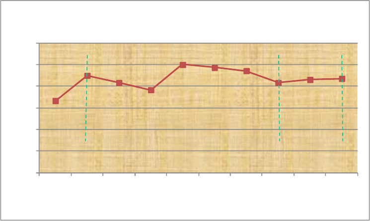
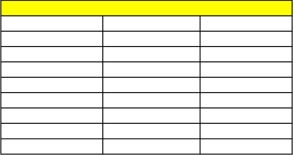
Perhaps a more effective way of displaying power or mass margin TPMs is graphically. Figure 3-16 is an
example of displaying the mass margins for a particular program/project. A similar plot can be developed
for power margin TPM.
Figure 3-16 Example Plot for Mass Margin Indicator
Date
Mass
Margin
Planned
Margin
Upper
Tol
Lower
Tol
Req. Goal
1/1/11 1 15 20 10 0 4
2/1/11 -2 14 19 10 0 4
3/1/11 -3 13 18 9 0 4
4/1/11 9 12 17 8 0 4
5/1/11 9 11 15 8 0 4
6/1/11 8 10 15 7 0 4
7/1/11 8 9 13 7 0 4
8/1/11 8 8 11 6 0 4
9/1/11 6 7 10 6 0 4
10/1/11 3 7 8 5 0 4
11/1/11 1 6 8 5 0 4
12/1/11 -2 6 7 5 0 4
1/1/2012 -3 5 7 4 0 4
2/1/2012 -2 5 6 4 0 4
3/1/2012 -1 4 5 4 0 4
4/1/2012 -1 4 4 4 0 4
-5
0
5
10
15
20
25
J
F
M
A
M
J
J
A
S
O
N
D
J
F
M
A
Mass Margin TPM
Mass
Planned
Upper Tol
Lower Tol
Req.
Goal
PDR
CDR
SIR
Mass
Scrub
32
3.7.3. Project-Unique TPMs
In addition to Common Leading Indicators, a program/project may need to identify other TPMs that are
unique to the particular type of program/project that is being conducted. For example, if the project is
avionics based, additional performance parameters such as bandwidth, pointing accuracy, and memory
usage may be important to track in order to ensure that the project is meeting its design requirements.
However, if the project is more mechanically based, these parameters may not be important/applicable,
but others such as stress, envelope size, or actuator force may be. There are many parameters that a
project can and will measure at some level. TPMs should be that selected subset that most affect the
design or performance of the program/project and should be tied to the Measures of Effectiveness and
Measures of Performance as described in NPR 7123.1 and NASA/SP-2007-6105, NASA Systems Engineering
Handbook.
Table 3-13 is an example of some other TPMs that the program/project may consider. The specific project
unique TPMs that the program/project decides to use should be documented in the Formulation
Agreement and the Program/Project Plan and/or the Systems Engineering Management Plan.
Table 3-13 Example Project-Unique TPMs
3.8. Manufacturing Trends
Manufacturing trends are intended to provide quantifiable evidence of potential technical problems,
monitor performance, and reveal the most important problems that affect a system that could
substantially affect cost, schedule, and quality and threaten a project’s success. During manufacturing,
nonconformances are typically documented and resolved using a Materials Review Board (MRB) process,
or its equivalent. Once non-conforming material or parts (items that fail inspection, i.e., are rejected) have
been identified, the MRB reviews them and determines whether the material or parts should be returned,
reworked/repaired, used “as is,” or scrapped. The MRB also identifies potential corrective actions for
implementation that would prevent future discrepancies.
Pointing error Database Size RF Link Margin
Data Storage Lines of code Torque Factor
Throughput Thrust Strength Factor
Memory available Time to restore Cooling capacity
Speed Fault Tolerance Range
Reliability Utilization MTBF
Human Factors Pointing Accuracy Specific Impulse
Response time Jitter Other Margins
Availability Propellant Control stability
Example Project-Unique TPMs
33
3.8.1. Why is the Leading Indicator Important?
Leading indicators are important so the manufacturing discipline can conduct analysis and trending on
component and system requirements, materials, controlled/critical processes, and production problems.
At the manufacturing stage of the life cycle, problems can quickly become critical path schedule drivers
with accompanying adverse cost impacts. Early warning indicators are needed to provide triggers for
project risk mitigation decisions. For example, a pattern of frequent inspection failures of a particular
vendor’s printed circuit boards might indicate a need to investigate and correct root cause(s) or change
vendors. A trend showing a high number of scrapped weldments might be the result of an inadequate
weld schedule. Such problems can slow down or even bring production work to a halt. Finding and
qualifying a new printed circuit board vendor or going back into research and development to tighten up a
weld schedule could impose serious cost and schedule penalties.
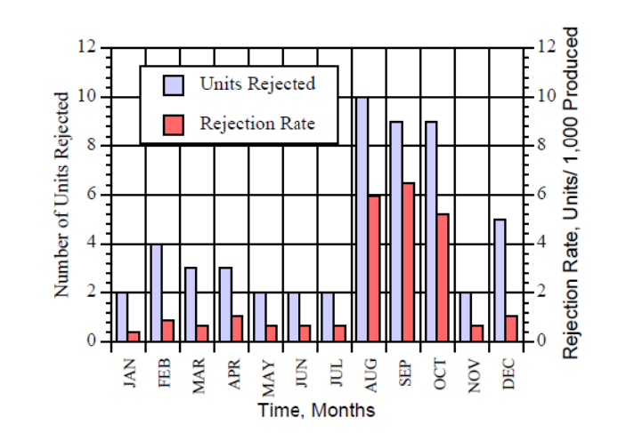
3.8.2. Number of MRB Non-conformance/Corrective Actions
The program/project should establish a measure of nonconformances as a function of time. Figure 3-17
shows an example of how this can be depicted. In this case, “units” could refer to piece parts of an
assembly or subassembly item.
Figure 3-17 Parts Rejection Rate over Time
Programs/projects should compare such information against production schedules. For example, the
number of rejected units should be assessed against both the actual and planned number of items in
manufacturing using the same time scale as the nonconformance metric. Trends in performance can be
identified by observing the percentages of non-conformances over time, looking for increases or
decreases.
34
The number of corrective actions initiated and implemented over time will provide an indication of the
health of the corrective action system. Measuring the initiation of corrective actions shows the quality
system’s sensitivity to deficiencies. Measuring implemented corrective actions and comparing them with
trends in non-conformances post-implementation would be an indicator of the effectiveness of the overall
manufacturing, quality control, and supply chain systems and risks.

35
Programmatic Leading Indicators
Like Technical Leading Indicators, Programmatic Leading Indicators are intended to provide program and
project personnel and Agency leaders with insight into cost, schedule, and staffing performance trends.
Sustained underperformance in these areas can result in project or program failure to meet internal or
external programmatic commitments. The indicators recommended here are intended to supplement
other reporting conventions and requirements that may be specified by other functional or programmatic
authorities.
4.1. Cost Trends
This category is intended to provide a longer temporal perspective than is sometimes provided in reporting
required by the owner of the cost function.
4.1.1. Why is the Leading Indicator Important?
Living within the internal and external cost commitments is becoming increasingly important. Stakeholders
are requiring more stringent cost and schedule control for projects. Since cost and schedule are so tightly
correlated, schedule growth frequently translates into cost growth. The earlier that cost and schedule
issues can be identified and addressed, the less the impact to total cost. With more effective cost and
schedule management, NASA can maximize the return on its investment of taxpayer resources.
4.1.2. Plan vs. Actual
Tracking the performance of actuals against the plan enables recognition of the potential impacts of
delayed receipt of funds and the effects of spending above or below the plan. Since most Centers,
programs, and project organizations will have preferred formats for tracking the cost and obligations
performance for the current year (year of execution), the leading indicator here proposes to track the
quarterly performance in obligations against multi-year plans for New Obligations Authority in both the
Agency Baseline Commitment (ABC) and the project Management Agreement as well as a multi-year cost
plan for the project. Analyzing current project Estimate at Completion (EAC) and life-cycle cost plans will
enable more immediate identification of potential issues that could affect the overall ABC. By monitoring
the extent to which either the Agency or project is unable to realize the basis for their commitments,
management will be encouraged to consider whether an adjustment in the agreements and recalculation
of confidence levels should be pursued.
The addition of quarterly reporting of actual costs against a multi-year cost plan will enable management
to regularly monitor any trends of ongoing expenditures, either in excess or below the plans that are tied
to the internal and external cost and schedule commitments. This perspective is often not regularly
reported in monthly project status reports.
As with the other leading indicators, the data may be displayed in either tabular or graphical form.
Examples are shown below.
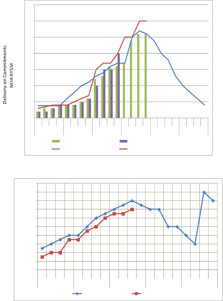
36
Figure 4-1 Management Agreement and ABC Plan vs. Actual
Figure 4-2 Commitment Cost Plan vs. Actual
0
5
10
15
20
25
30
35
Q1
Q2
Q3
Q4
Q1
Q2
Q3
Q4
Q1
Q2
Q3
Q4
Q1
Q2
Q3
Q4
Q1
Q2
Q3
Q4
Q1
Q2
Q3
Q4
FY09
FY10
FY11
FY12
FY13
FY14
Project Management Agreement
Management Agreement Realization
Agency Baseline Commitment
Realization
0
10
20
30
40
50
60
70
80
90
100
Q1
Q2
Q3
Q4
Q1
Q2
Q3
Q4
Q1
Q2
Q3
Q4
Q1
Q2
Q3
Q4
Q1
Q2
Q3
Q4
FY09
FY10
FY11
FY12
FY13
RY$M Cost
Commitment Cost Plan
Actual Costs
37
Table 4-1 Spreadsheet Example for Capturing Plan vs. Actual Measures
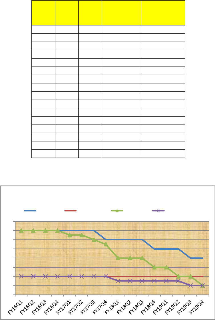
4.1.3. UFE
Measuring the use of cost margins—Unallocated Future Expenses (UFE)—against a plan enables
evaluation of time-phased releases in the context of the planned life-cycle activities and identified risks.
Utilization of UFE ahead of the anticipated needs and phasing may signal threats to the life-cycle cost
estimates or schedules, as it may indicate that identified risk mitigation needs have been underscoped,
that unidentified risks are being realized, that scope has been added, or baseline costs underestimated.
UFE plans and actuals should be measured for both project-managed and Agency-managed UFE.
Multi-year plans should incorporate local guidance or rules of thumb, and reporting should note reasons
for major releases or expenditures. Reporting may be done in either tabular or graphical form, as
illustrated in the examples below.
Plan Actual Plan Actual Plan Actual
FY16Q1 $100 $10 $80 $8 $20 $5
FY16Q2 $100 $40 $80 $35 $40 $30
FY16Q3 $100 $60 $80 $55 $60 $50
FY16Q4 $100 $100 $80 $80 $80 $65
FY17Q1 $200 $30 $170 $25 $30 $15
FY17Q2 $200 $60 $170 $55 $60 $40
FY17Q3 $200 $120 $170 $110 $130 $90
FY17Q4 $200 $200 $170 $170 $170 $150
FY18Q1 $300 $100 $270 $90 $50 $45
FY18Q2 $300 $300 $270 $200 $120 $115
FY18Q3 $300 $300 $270 $270 $220 $250
FY18Q4 $300 $300 $270 $270 $270 $275
FY19Q1 $200 $50 $180 $45 $40 $35
FY19Q2 $200 $100 $180 $90 $80 $75
FY19Q3 $200 $150 $180 $140 $150 $130
FY19Q4 $200 $180 $180 $180 $180 $180
Note: $M. Amounts are cumulative per year
Date
Cost
Mgmt Agreement
ABC NOA
38
Table 4-2 Example Spreadsheet for Project and Agency UFE Usage
Figure 4-3 UFE Burndown with Life-Cycle Review Notations
Date
PM UFE
Plan
Agency
UFE
Plan
PM UFE ($M)
Agency UFE
($M)
FY16Q1 70 20 $70 $20
FY16Q2 70 20 $70 $20
FY16Q3 70 20 $70 $20
FY16Q4 70 20 $70 $20
FY17Q1 70 20 $65 $20
FY17Q2 70 20 $65 $20
FY17Q3 70 20 $60 $20
FY17Q4 60 20 $55 $20
FY18Q1 60 20 $40 $15
FY18Q2 60 20 $40 $15
FY18Q3 60 20 $40 $15
FY18Q4 50 20 $30 $15
FY19Q1 50 20 $30 $15
FY19Q2 50 20 $20 $15
FY19Q3 40 20 $20 $10
FY19Q4 40 20 $10 $10
0
10
20
30
40
50
60
70
80
UFE Burndown($M)
PM UFE Plan Agency UFE Plan PM UFE ($M) Agency UFE ($M)
39
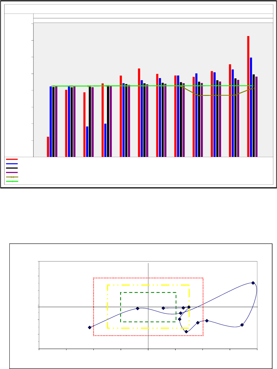
4.1.4. EVM
Earned Value Management (EVM) is one of the recognized methods of measuring integrated cost and
schedule performance against a plan. Based on the recorded performance to date, EVM will identify
variances, help identify trends, and predict resulting changes in the schedule and Estimate at Completion
(EAC). Traditionally reserved for application on contracts, NASA has extended EVM application to the
project level, taking in the integrated performance on multiple contracts and civil service efforts.
EVM establishes a baseline for measuring progress. That is, accomplishment (also known as Budgeted Cost
of Work Performed (BCWP) is compared to the Actual Cost of Work Performed (ACWP) to determine cost
variances and compared to the Budgeted Cost of Work Scheduled (BWCS) to identify schedule variances.
Additionally, the Cost Performance Index (CPI) and Schedule Performance Index (SPI) can be generated
from the Earned Value Measurement System. As shown in Figure 4-5, A CPI >1 indicates the project is
under-running costs, whereas a CPI<1 indicates an over-run. Likewise, a SPI >1 indicates the project is
ahead of schedule and an SPI <1 indicates being behind schedule. The EVMS provides trend analyses and
can generate a mathematical EAC, which can be compared to the Budgeted Estimate at Completion (BAC).
Several software packages (e.g., wInsight) will generate a series of mathematical EACs that can provide the
project with an estimated range of EAC possibilities based on trend information.
The graph below illustrates a trend analysis of the EAC, CPI, SPI, and the available/planned BAC. Although
the display below is an example of a contractor report and limited to a one-year period, the reported
elements are those intended for application at the project level. Reporting across multiple years is
expected. Early in the project, level of effort tasks can dominate and effectively cancel out useful reporting
on other elements, so if it is possible it is most desirable to report the results both with and without the
Level of Effort (LOE) elements.
40
Figure 4-4 Example Plot of EVM Parameters
The display below provides more insight into the variation of the CPI and SPI over time and the “bullseye”
provides at a glance interpretation of the performance.
Figure 4-5 EVM CPI vs. SPI Bullseye Chart Example
800
900
1,000
1,100
1,200
1,300
1,400
1,500
2007
OCT NOV DEC
2008
JAN FEB M AR APR M AY JUN JUL AU G SEP
Northrop Grumman Ship Systems N00024-04-2204 FPIF PROD
Element: 00000000 Name: Project LevelEAC / BAC
Dollars in Millions
CPI 3p Ave 1,4251,2551,2141,1791,1881,1981,2301,1871,1401,0871,102821
CPI 6p Ave 1,2951,2241,2071,2011,1881,1721,1601,1428998821,1211,122
CPI SPI 1,1941,1711,1591,1501,1481,1441,1411,1361,1291,1211,1171,118
CUM CPI 1,1811,1611,1511,1431,1421,1381,1351,1311,1261,1171,1211,122
K EAC 1,1121,0701,0691,0681,1261,1261,1261,1261,1261,1251,1251,125
BAC 1,1271,1271,1271,1261,1261,1261,1261,1261,1261,1251,1251,125
Cost/Schedule Performace
0.70
0.80
0.90
1.00
1.10
1.20
1.30
0.60 0.70 0.80 0.90 1.00 1.10 1.20 1.30 1.40
CPI
SPI
ANALYZE COST & SCHEDULE
CONSIDER RE-BASELINING
FAIR PLANNING &
PERFORMANCE
EXCELLENT PLANNING
&
PERFORMANCE
Nov
Dec
May
Jul
Jun
Apr
Oct
Over-running Costs
Ahead of Schedule
Over-running Costs
BehindSchedule
Under-running Costs
Ahead of Schedule
Under-running Costs
BehindSchedule
Jan
Mar
Feb
Aug
Sep
41
Earned Value reporting is most useful when the project baselines are stable. If there is a substantial
amount of flux in the baselines (either cost or schedule), the project earned value baseline may rapidly
become out of date and the reporting against an out of date baseline may be less than helpful. In those
instances, the project should provide alternative means of measuring integrated cost and schedule
performance.
4.2. Schedule Trends
4.2.1. Why is the Leading Indicator Important?
Tracking schedule trends over a multi-year horizon provides an easily interpreted means of measuring
progress. Because of the strong correlation between cost and schedule, schedule performance is a good
predictor of cost performance. Although current reporting practices provide current schedules, tracking
near term milestones within the current year, and a status on the use of schedule margins, the shortened
performance period does not provide a complete picture of total performance.
4.2.2. Critical path slack/float
The best reporting practices on the status of schedule margin and slack provide data against an anticipated
burndown or plan, along with acceptable ranges and explanations of major releases/uses of margin or
slack. Premature use of slack in the early phases of the life cycle may indicate the inability to deliver
products as planned. The first example below shows the actual performance against plan, identifies the
critical ranges of remaining slack, and provides primary reasons for the release or use of slack within a
single year.
Figure 4-6 Example of Project Schedule Slack vs. Plan
-5
5
15
25
35
45
Sep '04
Oct '04
Nov '04
Dec '04
Jan '05
Feb '05
Mar '05
Apr '05
May '05
Jun '05
Jul '05
Aug '05
Total Slack
Slack
Plan
Plan
Alert
Zone 1
Alert
Zone 2
Alert
Zone 3
Test chamber
availability delay
Troubleshoot
Noise anomaly
Replace cracked
DRX -002
WBS 1.1.2.2 RTT B Assembly Schedule Risk Indicator
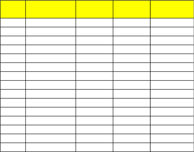
42
Ideally, the display would report against multiple years on the same trend lines as the tabular example
below.
Table 4-3 Spreadsheet Example for Capturing Schedule Slack
4.2.3. Critical Milestone Dates
It is equally important that the project provide a multi-year trend analysis of its overall schedule
achievement. The project should identify a limited number of significant predictive milestones and track
their achievement. The selection focuses on events that are key to delivering readiness for the life-cycle
phase or achieving the mitigation of a significant risk. That is, projects must go beyond major milestone
events and focus on the larger series of intermediate milestones and activities to understand progress
against the plan. These milestones typically would relate to drivers of risk or cost. The display should show
plan vs. actual achievements in a cumulative fashion over the planned development period. A quarterly
display is generally sufficient to provide a useful trend, as illustrated below.
Date
Total Sched
Slack (Months)
Planned
Milestones
Completed
Milestones
% Completed
Milestones
FY16Q1 20 0 0 0%
FY16Q2 20 1 0 0%
FY16Q3 15 3 1 5%
FY16Q4 15 4 3 15%
FY17Q1 15 5 5 25%
FY17Q2 12 6 5 25%
FY17Q3 12 8 5 25%
FY17Q4 12 9 6 30%
FY18Q1 9 10 6 30%
FY18Q2 9 11 7 35%
FY18Q3 9 12 8 40%
FY18Q4 4 13 9 45%
FY19Q1 4 14 11 55%
FY19Q2 2 15 12 60%
FY19Q3 2 16 13 65%
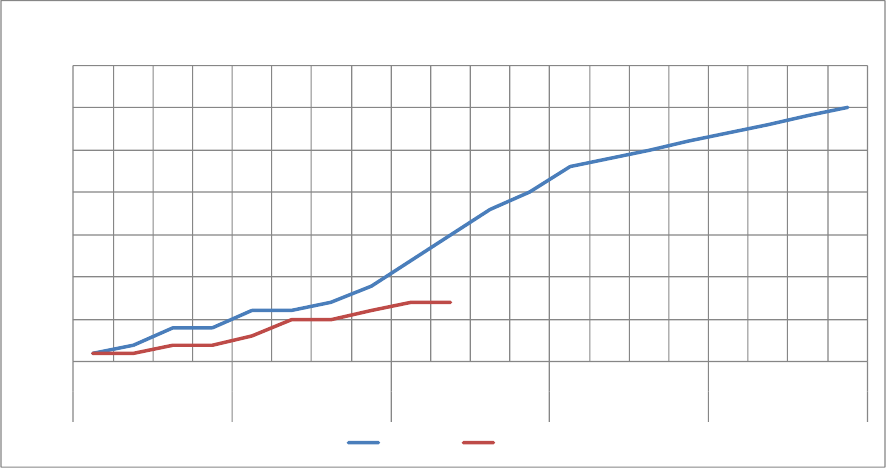
43
Figure 4-7 Cumulative Number of Milestones Planned in a Time Period vs. the Number Actually
Accomplished.
4.3. Staffing Trends
4.3.1. Why is the Leading Indicator Important?
The inability to properly staff positions may indicate an increased risk of not meeting cost and schedule
plans and could indicate product quality issues. Staffing trends should be reported for Civil Servant FTE and
Support Service Contractor WYE, as well as Prime Contractor WYE. It is important to monitor all three
staffing trends since it is sometimes possible to reassign work among available resources, e.g. Prime
Contractor to In-house. Current reporting practices are frequently limited to the execution year, but it is
most helpful to take a longer trend view of staffing.
In addition, since the majority of the cost associated with the development of hardware or software is the
cost of personnel, it is critical that staffing plans be monitored as a key indicator of whether the project is
heading in a direction that is likely to lead to a cost overrun. It is frequently useful to look at both labor
costs and FTE or WYE.
4.3.2. FTE/WYE Planned vs. Actual
Reporting staffing level plan vs. actuals can be handled in either tabular or graphical format. It may be
useful to provide a longer-term trend on a quarterly basis as a supplement to the reporting being done for
the year of execution. A tabular display example is provided in Table 4-4.
0
5
10
15
20
25
30
35
Q1
Q2
Q3
Q4
Q1
Q2
Q3
Q4
Q1
Q2
Q3
Q4
Q1
Q2
Q3
Q4
Q1
Q2
Q3
Q4
FY01
FY02
FY03
FY04
FY05
Cumulative Milestones
Key Milestones Plan v Actual
Cum Plans
Actuals
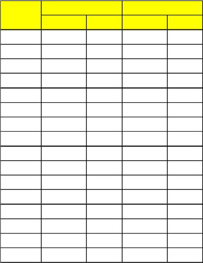
44
Table 4-4 FTE and WYE Staffing Levels Planned vs. Actual
4.3.3. Fully Integrated Staff Year Equivalent reporting
As noted, a fully integrated view can be useful in understanding why costs may be running either below or
ahead of plan and it can quickly identify questions that should be posed about the reassignment of work
and the related cost and schedule consequences. In the illustration below, it is apparent that the
instrument developers are running well behind plan, which should raise questions about the viability of the
planned schedule.
Planned Actual Planned Actual
FY16Q1 12.2 10.5 $450 $400
FY16Q2 12.5 11.5 $470 $450
FY16Q3 13.1 12.8 $470 $450
FY16Q4 13.1 12.9 $470 $470
FY17Q1 11.5 12.1 $480 $400
FY17Q2 12.3 12.3 $540 $480
FY17Q3 13.5 13.1 $540 $490
FY17Q4 13.5 13.2 $500 $520
FY18Q1 10.5 9.1 $400 $350
FY18Q2 11.2 10.5 $450 $420
FY18Q3 12.5 12.8 $450 $460
FY18Q4 12.6 12.8 $400 $410
FY19Q1 8.8 9.1 $300 $280
FY19Q2 9.5 9.2 $350 $330
FY19Q3 9.1 8.8 $300 $320
FY19Q4 8.5 8.6 $250 $260
Date
FTE
WYE $
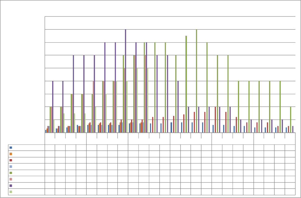
45
Figure 4-8 Example of Fully Integrated Staff Reporting
Q1
Q2
Q3
Q4
Q1
Q2
Q3
Q4
Q1
Q2
Q3
Q4
Q1
Q2
Q3
Q4
Q1
Q2
Q3
Q4
Q1
Q2
Q3
Q4
FY09
FY10
FY11
FY12
FY13
FY14
Plan CS
10
15
20
30
30
30
30
30
35
35
35
35
40
40
40
40
30
30
25
25
20
20
20
20
ACT CS
15
15
25
25
35
35
35
40
40
40
Plan SSC
25
25
25
25
40
40
40
50
50
50
60
60
65
70
80
80
100
80
60
40
40
40
25
25
ACT SSC
25
25
25
25
30
30
30
40
40
40
Plan Prime
100
100
150
150
150
200
200
300
300
350
350
350
300
375
400
350
300
300
200
200
200
200
200
100
ACT PRIME
100
100
150
150
200
200
200
250
300
300
Plan Instr vendors
200
200
300
300
300
350
350
400
350
350
300
300
200
100
100
100
100
100
50
50
50
50
50
25
ACT INSTR VENDOR
50
75
75
75
100
150
200
200
250
250
0
50
100
150
200
250
300
350
400
450
MYE
Planned vs Actual MYE

46
References
1. NASA/SP-2016-6105 “NASA Systems Engineering Handbook,” Rev 2 , 2016
2. “Systems Engineering Leading Indicators for Assessing Program and Technical Effectiveness,”
Donna H. Rhodes, Ricardo Valerdi, Garry J. Roedler. Massachusetts Institute of Technology and
Lockheed Martin Corporation. Reprint of an article accepted for publication in Systems
Engineering, 2008
3. “Systems Engineering Leading Indicators Guide,” Version 2.0, MIT, INCOSE and PSM joint paper,
2010
4. “Metric Guidebook for Integrated Systems and Product Development,” INCOSE, 1995
5. “Technical Measurement,” a Collaborative Project of PSM, INCOSE and Industry, 2005
6. BAE Presentation “Technical Performance Measure,” Jim Oakes, Rick Botta, and Terry Bahill, 2005
47
Appendix A Acronyms
ABC Agency Baseline Commitment
ACWP Actual Cost of Work Performed
BAC Budgeted Estimate at Completion
BCWP Budgeted Cost of Work Performed
CDR Critical Design Review
CPI Cost Performance Index
DR Discrepancy Report
EAC Estimate at Completion
EVM Earned Value Management
FTE Full-time Equivalent
ICD Interface Control Document
INCOSE International Council on System Engineering
MRB Material Review Board
NASA National Aeronautics and Space Administration
NOA New Obligation Authority
PDR Preliminary Design Review
PLI Programmatic Leading Indicator
PM Program or Project Management
PR Problem Report
PSM Practical Software and Systems Measurement
RFA Request For Action
RID Review Item Discrepancy
SAR System Acceptance Review
SDR System Definition Review
SEMP Systems Engineering Management Plan
SIR System Integration Review
SPI Schedule Performance Index
SRB Standing Review Board
SRR Systems Requirement Review
TBD To Be Determined
TBR To Be Resolved
TLI Technical Leading Indicator
TPM Technical Performance Measure
UFE Unallocated Future Expenditures
WYE Work Year Equivalent

48
Appendix B Glossary
Deviation: a documented agreement intentionally releasing a program/project from meeting a
requirement prior to the Implementation phases of the life cycle.
Leading Indicator: a measure for evaluating the effectiveness of how a specific activity is applied on a
program in a manner that provides information about impacts likely to affect the system performance
objectives. A leading indicator may be an individual measure or collection of measures predictive of future
system [and project] performance before the performance is realized. The goal of the indicators is to
provide insight into potential future states to allow management to act before problems are realized.
Technical Performance Measure: a critical or key performance parameter that is monitored by comparing
the current actual achievement of the parameter with that anticipated at the current time and on future
dates.
Verification: the proof of compliance with program/project requirements. This can be done through test,
analysis, demonstration, or inspection. Each requirement will need to be verified through one or more of
these methods.
Waiver: a documented agreement intentionally releasing a program/project from meeting a requirement
after reaching the Implementation phases of the life cycle.
49
Appendix C Summary of Common Indicators
Type
Indicator
Calculation
• Min. Graph Characteristics
Requirements
Trend
Requirement Growth
• Number of Requirements per document
and/or in total
• Percent growth (((Current number req)
– (previous number req))/(previous
number req)) x 100
• Show volatility of requirements over
time: Requirement growth vs. time or #
req vs. time
• Indicate key milestones for reference
• Include descriptions of key events
TBD/TBR Burndown
• Number of TBD/TBRs per document
and/or in total
• Show how TBD/TBRs are being resolved
over time: TBD/TBR burndown vs. time
or % closure vs. plan vs. time
• Indicate key milestones for reference
• Include descriptions of key events
Pending Req. Changes
• Number of pending requirement change
requests per document and/or in total
• Show pending requests for
requirement changes over time
• Indicate key milestones for reference
• Include descriptions of key events
Interface Trend
Interface
Documentation
approved/pending
• Number of Interface documents
approved/Total number of interface
documents x 100
• Show volatility of interfaces over time:
Interface growth vs. time or
# interfaces vs. time
• Indicate key milestones for reference
• Include descriptions of key events
TBD/TBR Burndown
• Number of TBD/TBRs per document
and/or in total
• Show how TBD/TBRs are being resolved
over time: TBD/TBR burndown vs. time
or % closure vs. plan vs. time
• Indicate key milestones for reference
• Include descriptions of key events
Pending Req. Changes
• Number of pending requirement change
requests per document and/or in total
• Show pending requests for interface
changes over time
• Indicate key milestones for reference
• Include descriptions of key events

50
Type
Indicator
Calculation
• Min. Graph Characteristics
Verification Trend
Verification Burndown
• Number of open verifications/Total
number of verifications x 100
• Show how verifications are being
resolved over time: open verification
burndown vs. time vs. plan or % closure
vs. plan vs. time
• Indicate key milestones for reference
• Include descriptions of key events
Number of
deviations/waivers
• Number of approved and pending
deviations/waivers
• Show approved and pending requests
for deviations/waivers over time as a
number or percentage
• Indicate key milestones for reference
• Include descriptions of key events
Review Trend
Open RFAs/RIDs/AIs per
Review
• Number of open comments/Total
number of comments x 100
• Show number of open review
RFAs/RIDs/AIs over time as a number
or percentage
• Indicate key milestones for reference
• Include descriptions of key events
Software-unique
Trend
Number of
requirements per
build/release vs. plan
• Number of software requirements for
each build or release
• Show number of requirements
accomplished for each build vs. planned
• Indicate key milestones for reference
• Include descriptions of key events
Problem
Report/Discrepancy
Report Trend
Open PR/DRs
• (Number of open PR/DRs/Total number
PR/DRs) x 100
• Show number of open PR/DRs over
time as a number or percentage
• Indicate key milestones for reference
• Include descriptions of key events

51
Technical
Performance
Measures
Mass Margin
• Measured/calculated mass margin
• Show how mass margins are being used
over time: margin vs. time vs. plan or
raw mass value vs. plan vs. time with
limits indicated
• Indicate key milestones for reference
• Include descriptions of key events
Power Margin
• Measure/calculated power margin
• Show how power margins are being
used over time: margin vs. time vs. plan
or raw power value vs. plan vs. time
with limits indicated
• Indicate key milestones for reference
• Include descriptions of key events
Project-unique
• Trending of other TPMs selected by
project
• Show trending of the project unique
TPMs over time
• Indicate key milestones for reference
• Include descriptions of key events
Cost Margin Trend
Expenditure of UFE
• UFE Release plan vs. actual
• Show multi-year plans for use of UFE
• Incorporate local guidance/rules of
thumb
• Track actual against plans
• Include description of major releases
Schedule Margin
Trend
Total slack time
• Schedule slack in appropriate units
(days, months)
• Track margin against plan
• Explain major releases/use
• Can include performance against
rules/exceptions

52
Cost Trend
PM Agreement NOA
• Project Management Agreement NOA
received
• Current Agreement vs. planned
• Detail by quarter for multiple years
• Indicate key milestones for reference
• Include descriptions of key events
Cost
• Actual costs incurred by
program/project
• Plan vs. Actual costs
• Detail by quarter for multiple years
• Indicate key milestones for reference
• Include descriptions of key events
EVM
• BCWS – Budgeted Cost of Work
Scheduled (AKA “Plan”)
• ACWP – Actual Cost of Work Performed
(AKA “Actuals)
• BCWP – Budgeted Cost of Work
Performed (AKA “Earned Value)
• CPI = BCWP/ACWP (If < 1, over-running
costs; if > 1, under-running costs)
• SPI = BCWP/BCWS (If <1, behind
schedule; if >1, ahead of schedule)
• EAC = Estimate at Completion of Project
• Include CPI, SPI and EAC
• Minimum of one-year, multiple years
preferred
• If possible, report without LOE
elements as well as total
• Include additional evaluations of
performance, e.g. non EVMS where
possible
• Indicate key milestones for reference
• Include descriptions of key events
Staffing Trend
FTE
• Civil servant charges to program/project
• Plot as FTE number and/or in
equivalent dollars
• Show as multi-year trend of plan vs.
actuals
• Indicate key milestones for reference
• Include descriptions of key events
WYE
• Contractor support–primes,
subcontractors, support contractors
• Plot as dollar equivalents
• Show as multi-year trend of plan vs.
actuals
• Indicate key milestones for reference
• Include descriptions of key events
53
Appendix D Additional Indicators to Consider
In addition to the common leading indicators described in this guide, many other indicators or
measurements can be selected for a program/project. Some examples are provided below:
• Requirements Trends
o Percent requirements approved
o Estimated impact of requirement changes
o Requirement defect profile
o Requirement defect density
o Requirement defect escapes
o Cycle time for requirement changes
o Requirement validation rate
o Percent requirements validated
o Number of requirements
o Requirement completion status
o Number of waivers/deviations
o Number of change request and closure status
o Requirement traceability
• Verification trends
o Verification rate
o Percent requirements verified
o Past due verifications
o Actual vs. planned closures
o Requirement verification by event
o Requirement liens
o Number of approved waivers
o Number of open waivers
o Potential waivers
o Waiver risk level
• Work product approval
o Work product approval rate
o Distribution of dispositions for work products
• Staffing trends
o Organizational turnover
o Costing profile
o Key staffing positions that need to be filled
o Performance variance at subsystem level
o Staffing in relation to SPI trends
o Workforce composition diversity
54
• Risk
o Risk exposure
o Present risk mitigations closed
o Percent risk mitigations overdue
• System design trends
o Interface trends
▪ Percent interface growth
▪ Interface defect profile
▪ Interface defect density
▪ Interface defect escapes
▪ Cycle time for interface changes
▪ Rate of convergence of interfaces
▪ Total number of interface requirements
▪ ICD changes
▪ Delays in baseline ICD
o Change request approval/closure rates
o Change request cycle time
o Change request priority density
o Complexity index
o Technology maturity
▪ Monitoring of breadboard, engineering models, simulations
▪ Technology opportunity exposure
▪ Technology obsolescence
▪ TRL level maturity per plan
o Use of heritage systems
o Risk exposure trend
o Drawing/model maturity
• Process compliance
o Percent processes with discrepancies
o High risk processes
• Software Trends
o Change requests
o Facility development (testbeds)
o Software code Peer Review comment count
o SW milestone status
o SW plan vs. release
o SW module planned vs. actual completions
o Margin management on constrained resources
o Requirements allocation to software components & builds
o Software size in terms of Source Lines of Code or function points
o Software development effort in terms of staff hours or staff months
55
o Software development staffing in terms of actual staffing vs. planned staffing and staff
turnover
o Software development schedule start and completion dates
o Progress for detailed activities tracked against baseline plans
o Software defects
o Defect resolution effort in staff hours or staff months
o Defect resolution schedule start and completion dates
o Progress for defect resolution tracked against baseline plans
• Manufacturing trends
o Released for manufacturing
o Number of nonconformances that are opened, closed, resolved
o Number of open/closed inspection reports vs. time
• Facility and equipment availability
o Facility availability
o Equipment availability
• Review trends
o Action item closure performance
o Closure disposition distribution
o Number of document comments
o RFA status (open, closed, overdue)
• Cost/Schedule Trends
o Affordability
o Cost/schedule pressure
o Joint Confidence Level
o Replans
o Variance explanations
o Past performance UFE vs. Center guidelines
o Liens
o Threats
o Estimate at completion
o Time between schedule milestones
o Late task finishes
o Received/delivered products actual vs. plan
o SRA
o Cost of missions in extended operations
o Cost increase due to external forces (Continuing resolutions, new requirements, etc.)
o International partnership performance
• Other
o EEE parts approval
o Parts procurement and delivery trend
o Reliability analysis actual vs. planned completions
56
o Open design analysis discrepancy completion
o Completion of certification of flight readiness (CoFR) items vs. plan
o Number of drawing planned vs. actual over time
o Hardware build statue
o Problems, issues, and concerns over time
o Contract value
o Contract mods metrics
o Supplier and supply chain management
o Production metrics
o Contractor/subcontractor performance ratings
o Key programmatic and technical risk
o TRL levels planned vs. actual
o Risk status/mitigation implementation
